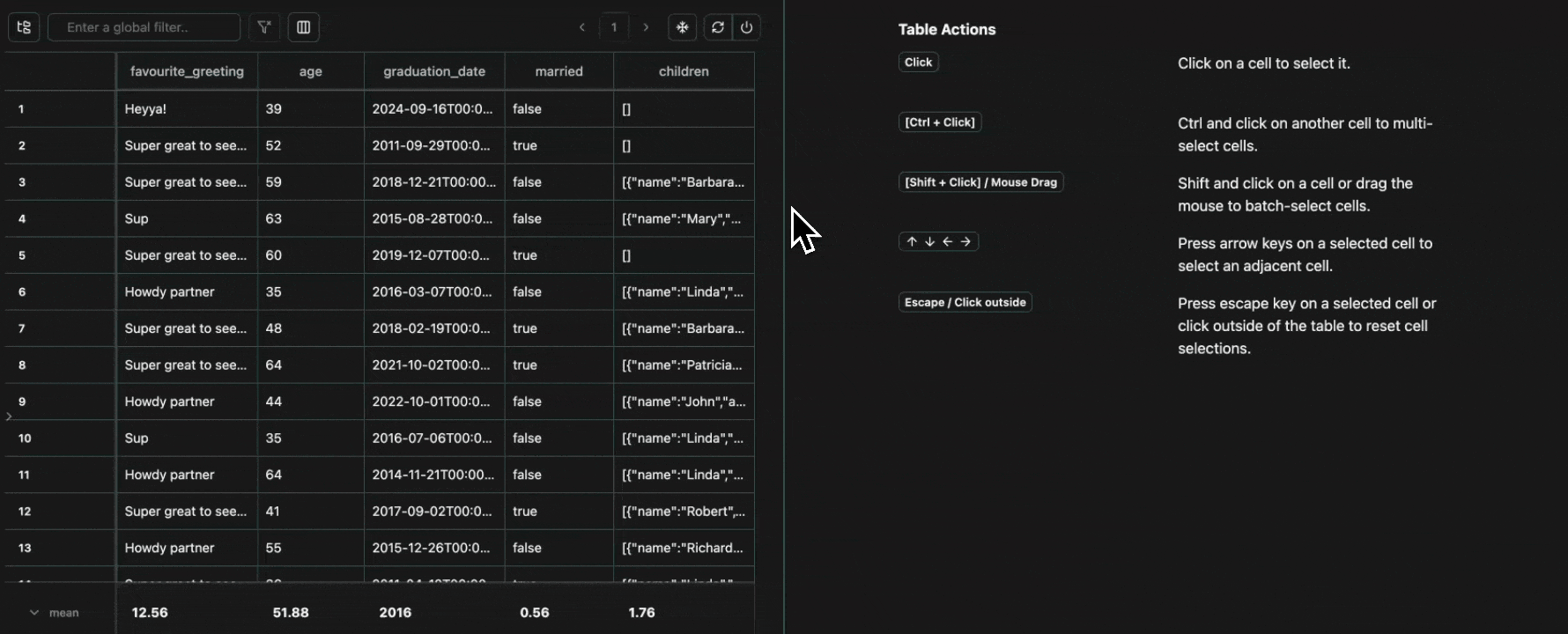
Expand
Expand
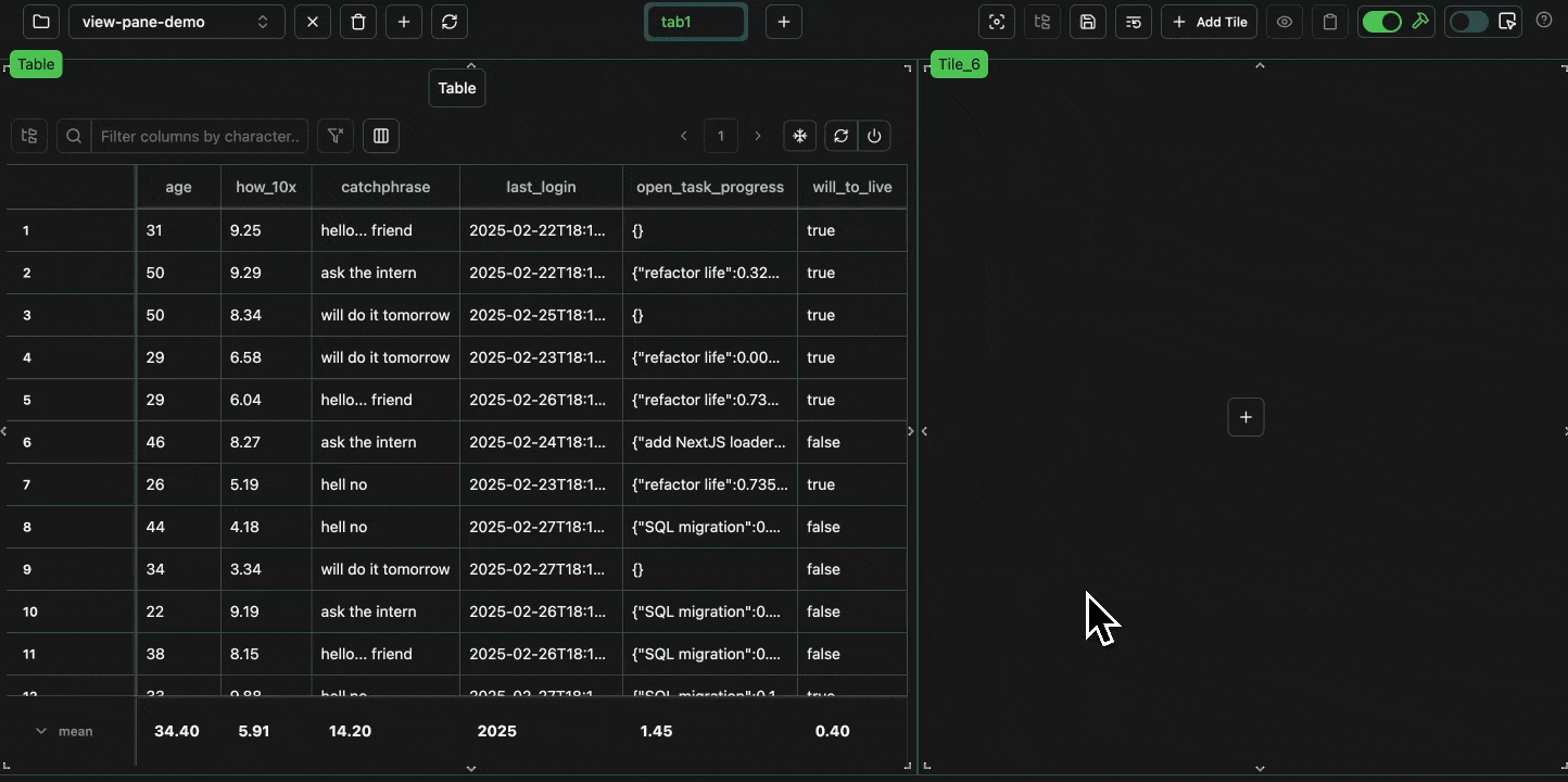 click image to maximize
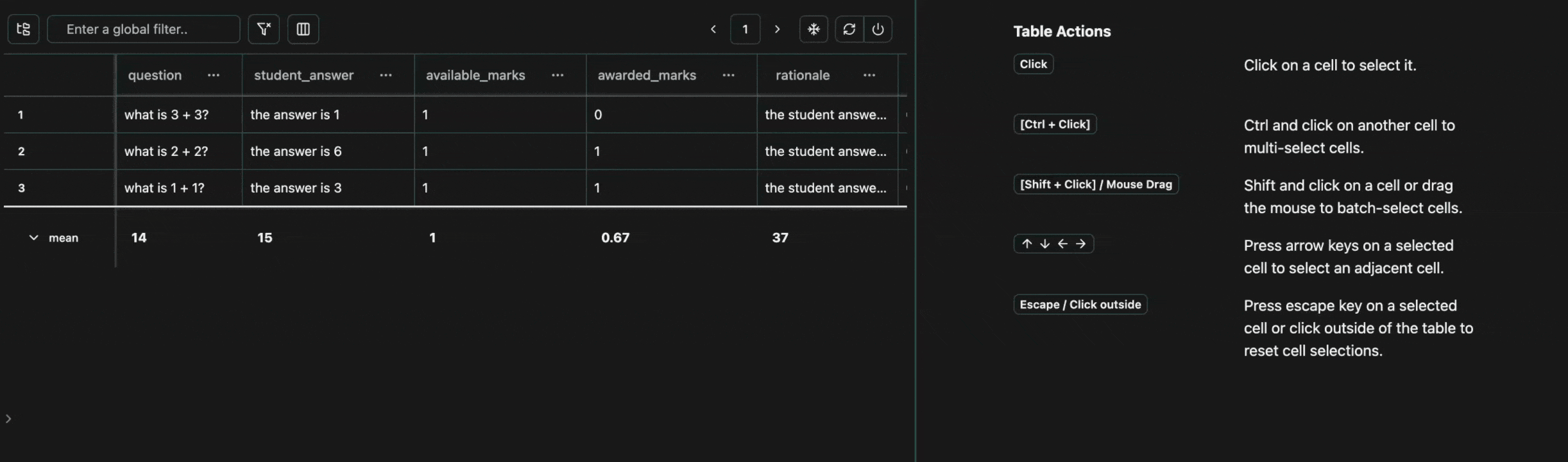
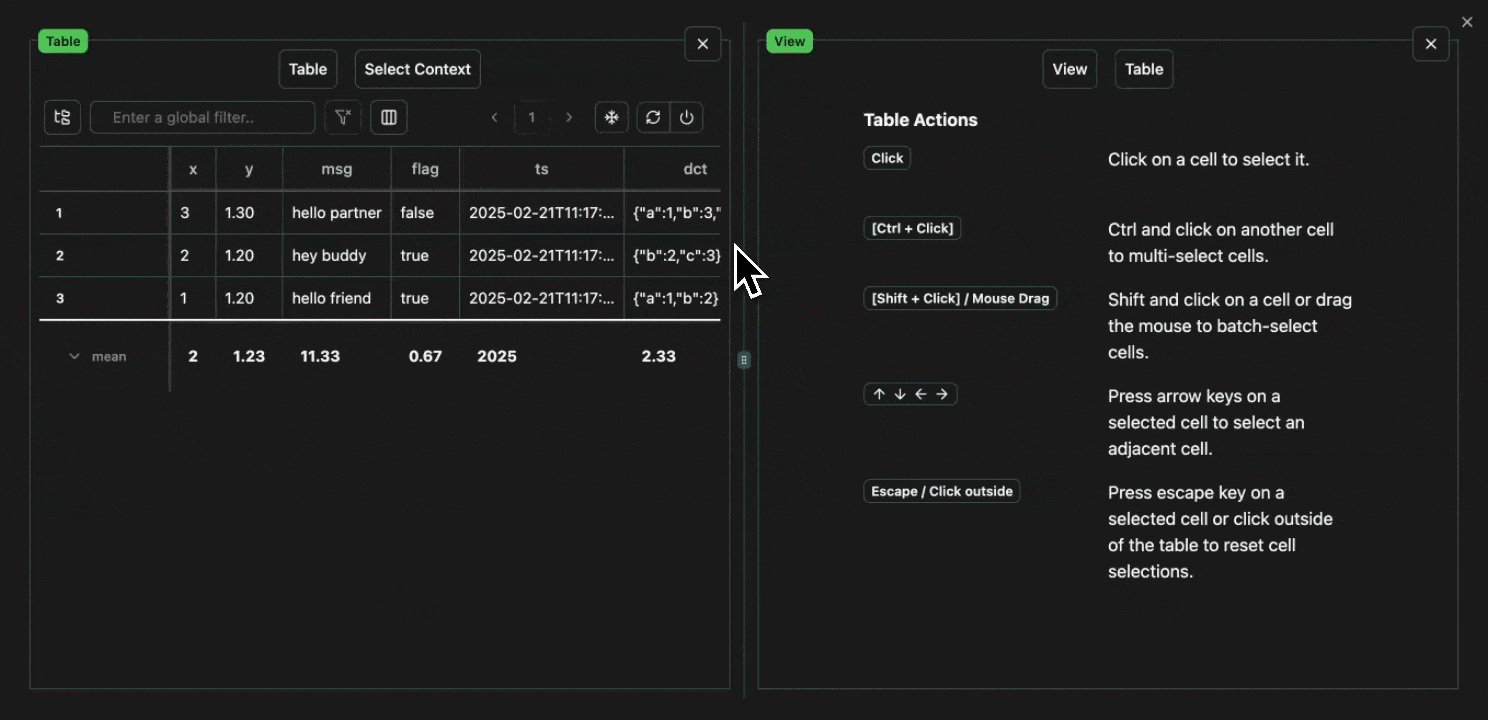
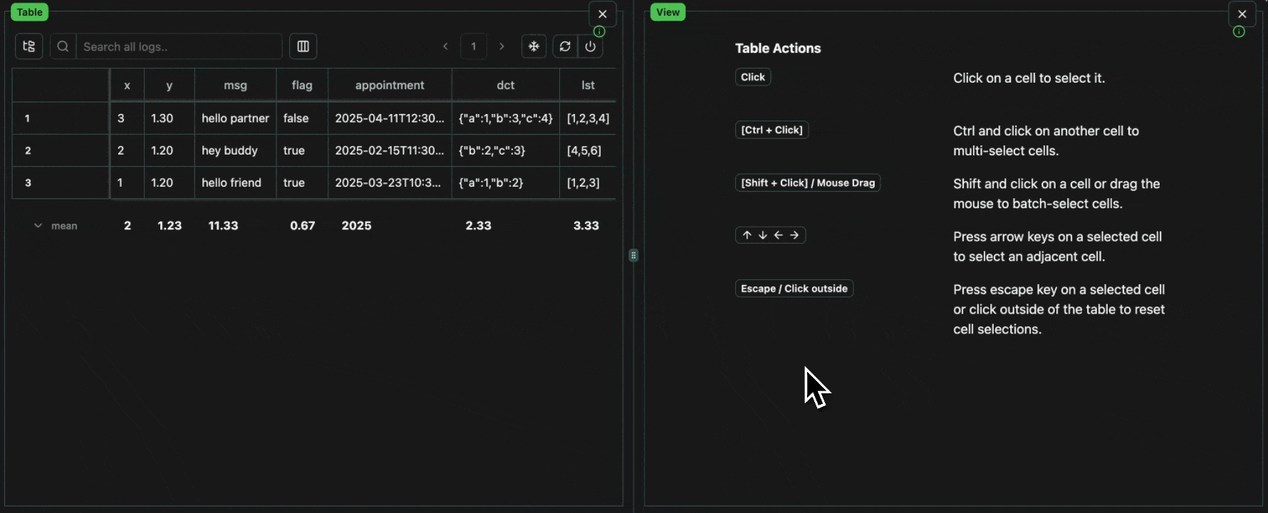
Cell Selection
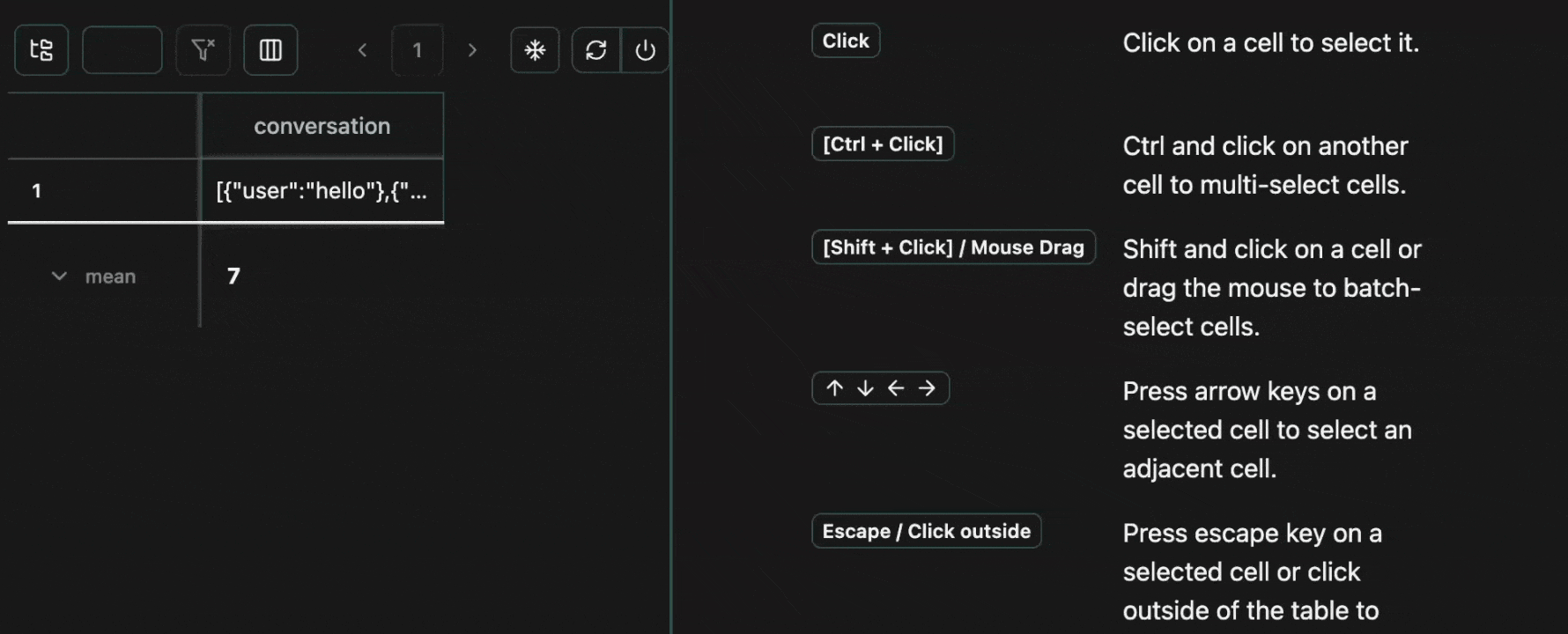
Every cell in a table is an atomic unit, which can be viewed independently. In it’s most basic form, the view pane acts as an expressive viewer for whatever cell(s) are selected in the table. These cells can be part of the same row, different rows, different columns, or any combination. In all cases, all of the data will be shown in the view pane.Expand
Expand
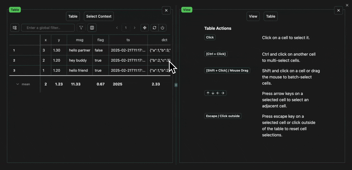
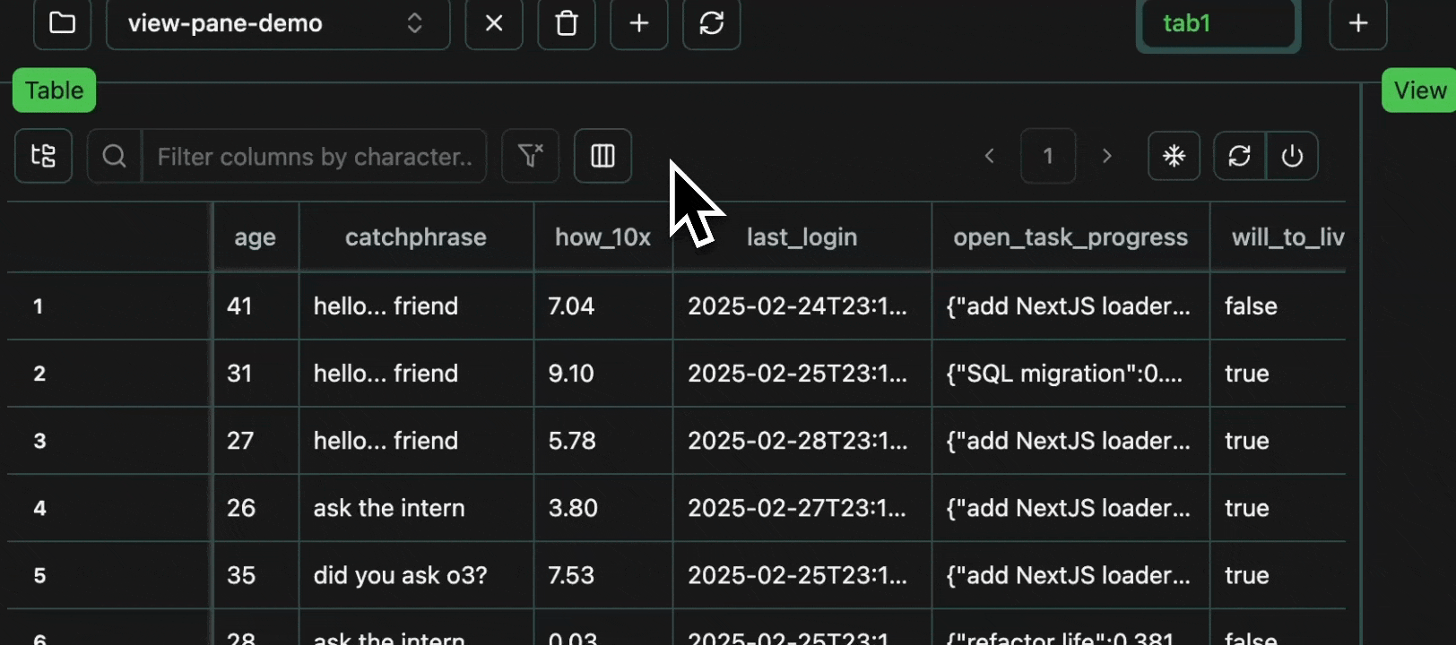 click image to maximize
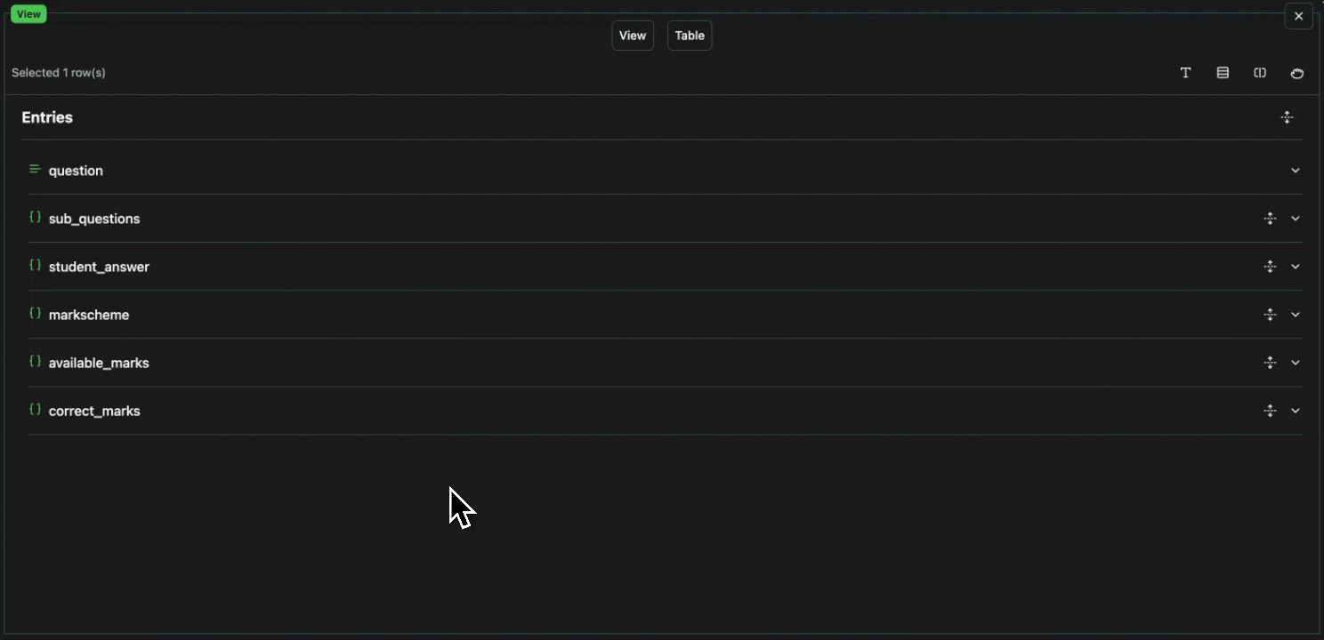
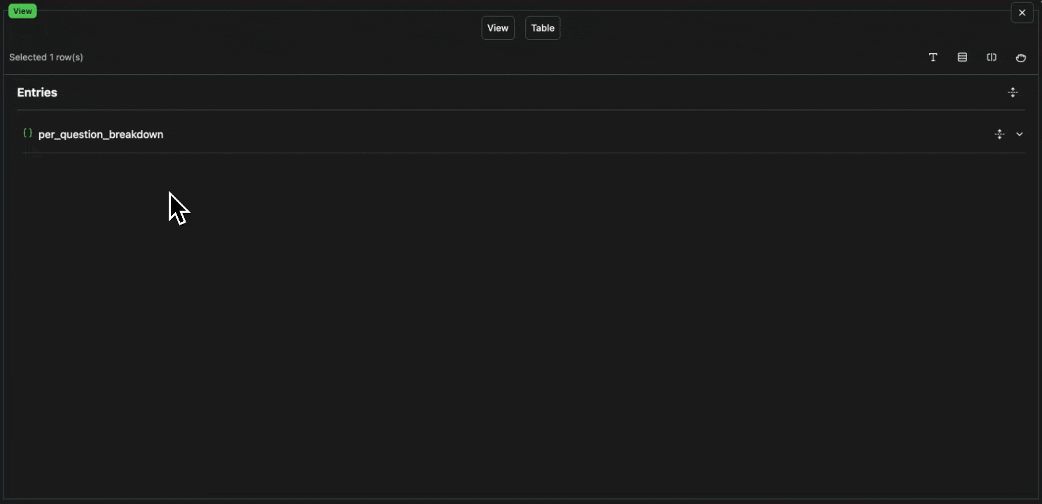
Grouping
To avoid redundancy, every value that is shared across multiple cells is grouped in the view pane, with all the row numbers shown at the top.Expand
Expand
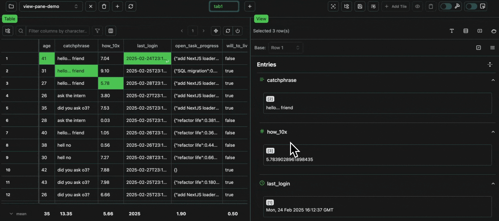 click image to maximize
View Modes
The view pane supports 3 different view modes:- Markdown: All text is rendered as markdown.
- Plain Text: All text is rendered as plain text.
- Raw: The columns (incuding dicts, lists, numbers etc.) are rendered as a raw strings, with no formatting or nested structure.
Expand
Expand
 click image to maximize
Hiding Columns
Columns can be hidden by directly clicking the (-) icon which appears on hover, and also via the show / hide selector menu at the top. Column hiding in the view pane is totally independent from hidden columns in the table, making it easy to split the data across the two formats. For example, consider the following logged data: Open in your consoleExpand
Expand
 click image to maximize
Moving Columns
Columns can easily be moved in the view pane by selecting drag mode and then simply clicking and dragging them.Expand
Expand
 click image to maximize
Split View
Sometimes it’s more convenient to view the data side-by-side, the split view makes this easy. You can toggle between one, two and three views.Expand
Expand
 click image to maximize
Nesting
By default, the view pane will only expand one nest level at a time. The deeper contents of dicts and lists are lazily loaded as the nest is incrementally expanded. Pressing “Expand All Children” will expand all children recursively with one click, and “Collapse All Children” will do the inverse.Expand
Expand
 click image to maximize
Diffs
The view pane supports very expressive diffs across cells. Let’s use a simple example for exploring the different diff features. Open in your consoleStrings
For string diffs, there are four modes:- None: No diff applied, just show contents grouped by value (as above).
- Lines: Per line diffs.
- Side-by-side: Per word diffs.
- Characters: Per character diffs.
Expand
Expand
 click image to maximize
Numeric
Numeric value “diffs” support the four basic operators:-, +, * and /.
Expand
Expand
 click image to maximize
DateTime
Datetime diffs are presented as a relative difference in time, in the appropriate units (weeks, days, seconds, miliseconds etc.)Expand
Expand
 click image to maximize
Structure Diffs
Aside from presenting the diffs for individual items, we can also see how the nested structure of dictionaries and lists change across logs. The same is also true for traces (more details below).Expand
Expand
 click image to maximize
Base Log
All diffs are relative to the selected base log. This base log can easily be changed at the top of the view pane.Expand
Expand
 click image to maximize
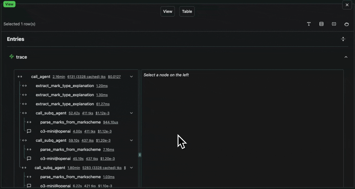
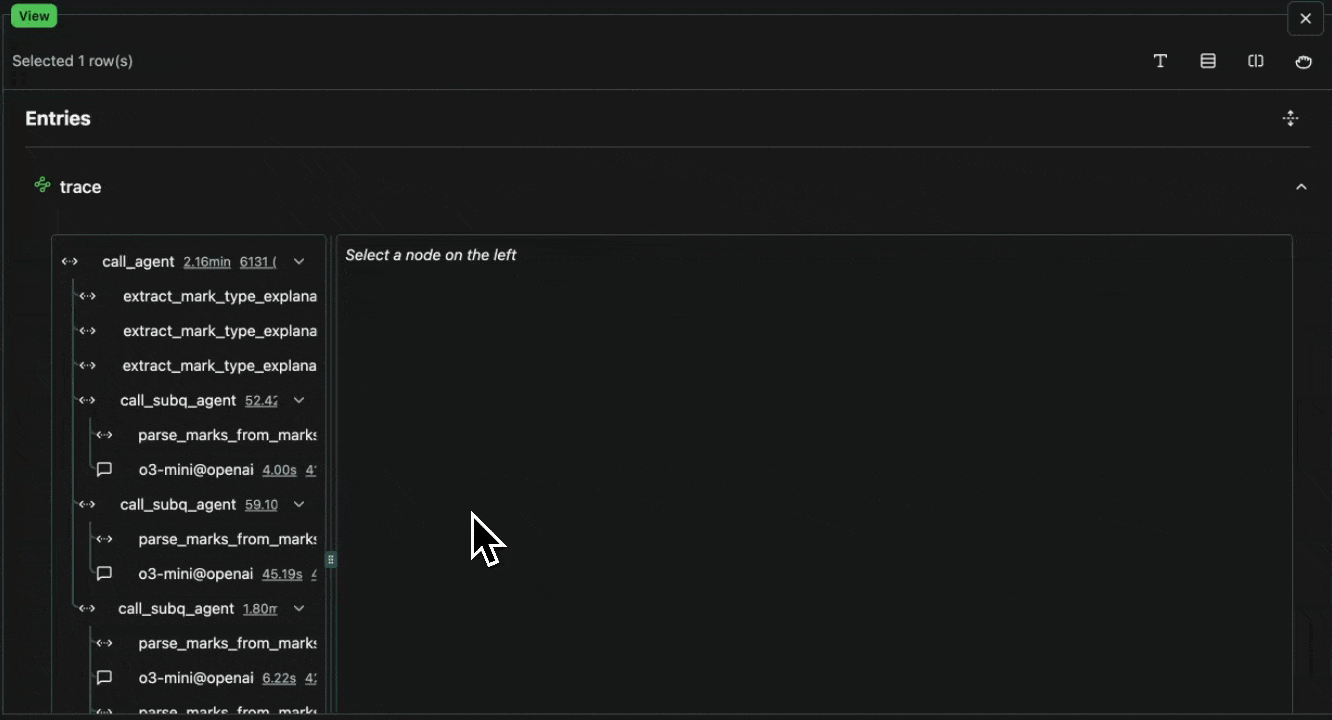
Traces
Last but not least, no observability tool would be complete without expressive traces. Traces enable you to get a complete view of nested function calls from your program 🔍Trace Viewer
The trace viewer is shown on the left, which shows the nested structure of your entire trace. Each item in the trace is a span (unit of computation), and the children of each span are shown nested underneath. Each span shows the cumulative values for:- Cost: Can be manually specified during tracing for arbitrary programs. Unify’s LLM clients automatically populate this based on the cost of the LLM calls.
- Tokens: Can be manually specified during tracing when integrating with other LLM providers. Unify’s LLM clients automatically populate this based on the tokens used in the LLM calls.
- Runtime: Tracked automatically during tracing of the program.
Expand
Expand
 click image to maximize
Span Viewer
The span viewer is shown on the right, and for each span, this shows:- Inputs: All inputs to the function call (if any).
- Outputs: All outputs from the function call (if any).
- Code: The source code of the function call.
- Execution Time: The time taken to execute the function call.
- Cost: The cost of the function call, including and excluding cached LLM calls which didn’t cost anything during the trace itself, but would if there was no cache to read from.
- ID: The unique identifier for the span.
Expand
Expand
 click image to maximize
Expand
Expand
 click image to maximize